library(tidyverse)
library(magrittr)

link_list_dk <- list(
  "1996_atc_code_data.txt" = "https://medstat.dk/da/download/file/MTk5Nl9hdGNfY29kZV9kYXRhLnR4dA==",
  "1997_atc_code_data.txt"  = "https://medstat.dk/da/download/file/MTk5N19hdGNfY29kZV9kYXRhLnR4dA==",
  "1998_atc_code_data.txt" = "https://medstat.dk/da/download/file/MTk5OF9hdGNfY29kZV9kYXRhLnR4dA==",
  "1999_atc_code_data.txt" = "https://medstat.dk/da/download/file/MTk5OV9hdGNfY29kZV9kYXRhLnR4dA==",
  "2000_atc_code_data.txt" = "https://medstat.dk/da/download/file/MjAwMF9hdGNfY29kZV9kYXRhLnR4dA==",
  "2001_atc_code_data.txt" = "https://medstat.dk/da/download/file/MjAwMV9hdGNfY29kZV9kYXRhLnR4dA==",
  "2002_atc_code_data.txt" = "https://medstat.dk/da/download/file/MjAwMl9hdGNfY29kZV9kYXRhLnR4dA==",
  "2003_atc_code_data.txt" = "https://medstat.dk/da/download/file/MjAwM19hdGNfY29kZV9kYXRhLnR4dA==",
  "2004_atc_code_data.txt" = "https://medstat.dk/da/download/file/MjAwNF9hdGNfY29kZV9kYXRhLnR4dA==",
  "2006_atc_code_data.txt" = "https://medstat.dk/da/download/file/MjAwNl9hdGNfY29kZV9kYXRhLnR4dA==",
  "2007_atc_code_data.txt" = "https://medstat.dk/da/download/file/MjAwN19hdGNfY29kZV9kYXRhLnR4dA==",
  "2008_atc_code_data.txt" = "https://medstat.dk/da/download/file/MjAwOF9hdGNfY29kZV9kYXRhLnR4dA==",
  "2009_atc_code_data.txt" = "https://medstat.dk/da/download/file/MjAwOV9hdGNfY29kZV9kYXRhLnR4dA==",
  "2010_atc_code_data.txt" = "https://medstat.dk/da/download/file/MjAxMF9hdGNfY29kZV9kYXRhLnR4dA==",
  "2011_atc_code_data.txt" = "https://medstat.dk/da/download/file/MjAxMV9hdGNfY29kZV9kYXRhLnR4dA==",
  "2012_atc_code_data.txt" = "https://medstat.dk/da/download/file/MjAxMl9hdGNfY29kZV9kYXRhLnR4dA==",
  "2013_atc_code_data.txt" = "https://medstat.dk/da/download/file/MjAxM19hdGNfY29kZV9kYXRhLnR4dA==",
  "2014_atc_code_data.txt" = "https://medstat.dk/da/download/file/MjAxNF9hdGNfY29kZV9kYXRhLnR4dA==",
  "2015_atc_code_data.txt" = "https://medstat.dk/da/download/file/MjAxNV9hdGNfY29kZV9kYXRhLnR4dA==",
  "2016_atc_code_data.txt" = "https://medstat.dk/da/download/file/MjAxNl9hdGNfY29kZV9kYXRhLnR4dA==",
  "2017_atc_code_data.txt" = "https://medstat.dk/da/download/file/MjAxN19hdGNfY29kZV9kYXRhLnR4dA==",
  "2018_atc_code_data.txt" = "https://medstat.dk/da/download/file/MjAxOF9hdGNfY29kZV9kYXRhLnR4dA==",
  "2019_atc_code_data.txt" = "https://medstat.dk/da/download/file/MjAxOV9hdGNfY29kZV9kYXRhLnR4dA==",
  "2020_atc_code_data.txt" = "https://medstat.dk/da/download/file/MjAyMF9hdGNfY29kZV9kYXRhLnR4dA==",
  "2021_atc_code_data.txt" = "https://medstat.dk/da/download/file/MjAyMV9hdGNfY29kZV9kYXRhLnR4dA==",
  "2022_atc_code_data.txt" = "https://medstat.dk/da/download/file/MjAyMl9hdGNfY29kZV9kYXRhLnR4dA==",
  "atc_code_text.txt" = "https://medstat.dk/da/download/file/YXRjX2NvZGVfdGV4dC50eHQ=",
  "atc_groups.txt" = "https://medstat.dk/da/download/file/YXRjX2dyb3Vwcy50eHQ=",
  "population_data.txt" = "https://medstat.dk/da/download/file/cG9wdWxhdGlvbl9kYXRhLnR4dA=="
)

# ATC codes are stored in files
seq_atc <- c(1:26)
atc_code_data_list <- link_list_dk[seq_atc]

# drugs names
eng_drug <- read_delim(link_list_dk[["atc_groups.txt"]], delim = ";", col_names = c(paste0("V", c(1:6))), col_types = cols(V1 = col_character(), V2 = col_character(), V3 = col_character(), V4 = col_character(), V5 = col_character(), V6 = col_character())) %>%
  # keep drug classes labels in English
  filter(V5 == "1") %>%
  select(ATC = V1,
         drug = V2,
         unit_dk = V4)

# drugs data
atc_data <- map(atc_code_data_list, ~read_delim(file = .x, delim = ";", trim_ws = T, col_names = c(paste0("V", c(1:14))), col_types = cols(V1 = col_character(), V2 = col_character(), V3 = col_character(), V4 = col_character(), V5 = col_character(),V6 = col_character(), V7 = col_character(), V8 = col_character(), V9 = col_character(), V10 = col_character(), V11 = col_character(), V12 = col_character(), V13 = col_character(), V14 = col_character()))) %>%
  # bind atc_data from all years
  bind_rows()

# population data
pop_data <- read_delim(link_list_dk[["population_data.txt"]], delim = ";", col_names = c(paste0("V", c(1:7))), col_types = cols(V1 = col_character(), V2 = col_character(), V3 = col_character(), V4 = col_character(), V5 = col_character(), V6 = col_character(), V7 = col_character())) %>%
  # rename and keep columns
  select(year = V1,
         region_text = V2,
         region = V3,
         gender = V4,
         age = V5,
         denominator_per_year = V6) %>%
  # human-reading friendly label on sex categories
  mutate(
      gender_text = case_when(
      gender == "1" ~ "men",
      gender == "2" ~ "women",
      T ~ as.character(gender)
    )
  ) %>%
  # make numeric variables
  mutate_at(vars(year, age, denominator_per_year), as.numeric) %>%
  arrange(year, age, region, gender)

atc_data %<>%
  # rename and keep columns
  rename(
    ATC = V1,
    year = V2,
    sector = V3,
    region = V4,
    gender = V5, # 0 - both; 1 - male; 2 - female; A - age in categories
    age = V6,
    number_of_people = V7,
    patients_per_1000_inhabitants = V8,
    turnover = V9,
    regional_grant_paid = V10,
    quantity_sold_1000_units = V11,
    quantity_sold_units_per_unit_1000_inhabitants_per_day = V12,
    percentage_of_sales_in_the_primary_sector = V13
  )

atc_data %<>%
  # clean columns names and set-up labels
  mutate(
    year = as.numeric(year),
    region_text = case_when(
      region == "0" ~ "DK",
      region == "1" ~ "Region Hovedstaden",
      region == "2" ~ "Region Midtjylland",
      region == "3" ~ "Region Nordjylland",
      region == "4" ~ "Region Sjælland",
      region == "5" ~ "Region Syddanmark",
      T ~ NA_character_
    ),
    gender_text = case_when(
      gender == "0" ~ "both sexes",
      gender == "1" ~ "men",
      gender == "2" ~ "women",
      T ~ as.character(gender)
    )
  ) %>%
  mutate_at(vars(turnover, regional_grant_paid, quantity_sold_1000_units, quantity_sold_units_per_unit_1000_inhabitants_per_day, number_of_people, patients_per_1000_inhabitants), as.numeric) %>%
  select(-V14) %>%
  filter(
  region == "0",
  sector == "0",
  gender == "2"
)

atc_data %<>%
  # deal with non-numeric age in groups
  filter(
    str_detect(age, "[0-9][0-9][0-9]")
  ) %>%
  mutate(
    age = parse_number(age)
  ) %>%
  select(year, ATC, gender, age, number_of_people, patients_per_1000_inhabitants, region_text, gender_text)

regex_pregabalin <- "^N02BF02$"

atc_data %<>% filter(str_detect(ATC, regex_pregabalin))
atc_data %<>% left_join(eng_drug)
atc_data %<>% left_join(pop_data)

# group to the same categories as in Swedish data
atc_data_se <- readxl::read_xlsx(path = "C:/Users/au595736/OneDrive - Aarhus Universitet/ISPOR 2023/Statistikdatabasen_2023-03-15 10_54_00.xlsx", sheet = 1) %>%
  pivot_longer(cols = c("2006":"2022")) %>%
  mutate(
    name = as.numeric(name),
    country = "Sweden"
  )

atc_data %<>% mutate(
  age_cat = cut(age, c(-Inf, 14, 19, 24, 29, 34, 39, 44, 49, Inf))
) %>%
  group_by(age_cat, year) %>%
  mutate(
    number_of_people_age_cat = sum(number_of_people),
    denominator_per_year_age_cat = sum(denominator_per_year),
    patients_per_1000_inhabitants_age_cat = (number_of_people_age_cat/denominator_per_year_age_cat)*1000
  ) %>%
  ungroup() %>%
  filter(
    age_cat != "(-Inf,14]",
    age_cat != "(49, Inf]"
  ) %>%
  mutate(
    age_cat = case_when(
      age_cat == "(14,19]" ~ "15-19",
      age_cat == "(19,24]" ~ "20-24",
      age_cat == "(24,29]" ~ "25-29",
      age_cat == "(29,34]" ~ "30-34",
      age_cat == "(34,39]" ~ "35-39",
      age_cat == "(39,44]" ~ "40-44",
      age_cat == "(44,49]" ~ "45-49"
    ),
    country = "Denmark"
  ) %>%
  distinct(age_cat, year, number_of_people_age_cat, denominator_per_year_age_cat, patients_per_1000_inhabitants_age_cat)

atc <- full_join(atc_data, atc_data_se, by = c("year" = "name", "age_cat" = "Ålder", "patients_per_1000_inhabitants_age_cat" = "value", "country" = "country")) %>%
  select(year, age_cat, patients_per_1000_inhabitants_age_cat, country)

ggplot <- atc %>%
  # filter(!is.na(patients_per_1000_inhabitants_age_cat)) %>%
  mutate(label = if_else(year == 2022, as.character(age_cat), NA_character_),
         value = case_when(
             age_cat == "30-34" ~"#3E9286",
             age_cat == "35-39" ~ "#E8B88A",
             T ~ "gray"
         )) %>%
  ggplot(aes(x = year, y = patients_per_1000_inhabitants_age_cat, group = age_cat, color = value)) +
  geom_line() +
  facet_grid(cols = vars(country), scales = "free", drop = F) +
  theme_light(base_size = 14, base_family = "Ubuntu") +
  scale_x_continuous(breaks = c(seq(2004, 2022, 5))) +
  scale_color_identity() +
  theme(plot.caption = element_text(hjust = 0, size = 10),
        legend.position = "none",
        panel.spacing = unit(0.8, "cm")) +
  labs(y = "Female patients of reproductive age\nper 1,000 women in the population", title = "Pregabalin utilization in women", subtitle = "aged between 15 and 49 years in DK and SE\n2004-2022", caption = "Elena Dudukina | @evpatora") +
    ggrepel::geom_label_repel(aes(label = label), na.rm = TRUE, nudge_x = 3, hjust = 0.5, direction = "y", segment.size = 0.1, segment.colour = "black", show.legend = F, family = "Ubuntu")

ggsave(filename = paste0(Sys.Date(), "_pregabalin use in DK and SE.pdf"), plot = ggplot, path = "C:/Users/au595736/OneDrive - Aarhus Universitet/ISPOR 2023/", dpi = 900, height = 6, width = 8, device = cairo_pdf)Prenatal Exposure to Antiseizure Medication and Risk of Neurodevelopmental Outcomes: evidence from the Nordics
ISPOR-AU General Meeting, March 2023
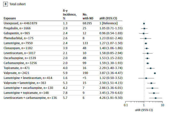
Previous results from the Nordics
No increased risks were identified for levetiracetam, gabapentin, pregabalin, or phenobarbital
Topiramate and valproate in monotherapy were associated with a 2- to 4-fold increased risk of autism spectrum disorders and intellectual disability1
Further questions
Use of active comparators for most used antiepileptic medication: pregabalin
Exposure unrestricted to mono-therapy (any prenatal exposure to pregabalin)
 vs
vs 
Pregabalin indications
Approved indications for pregabalin (in the European Union):
Epilepsy
Neuropathic pain
Generalized anxiety disorder (GAD)


Previous evidence on prenatal pregabalin exposure and adverse outcomes
- European Network of Teratology Information Services (ENTIS):
- 3-fold increased risk of any major non-chromosomal congenital malformation
- Medicaid beneficiaries + MarketScan in the US:
- Pooled RR=1.33 (95% CI: 0.83-2.15); interpreted as no association
- Confounding by indication is a major concern since most of the earlier studies compared exposure to pregabalin with no exposure to AED
- Postnatal outcomes are rarely investigated
- Particular postnatal outcomes are of interest, eg, ADHD

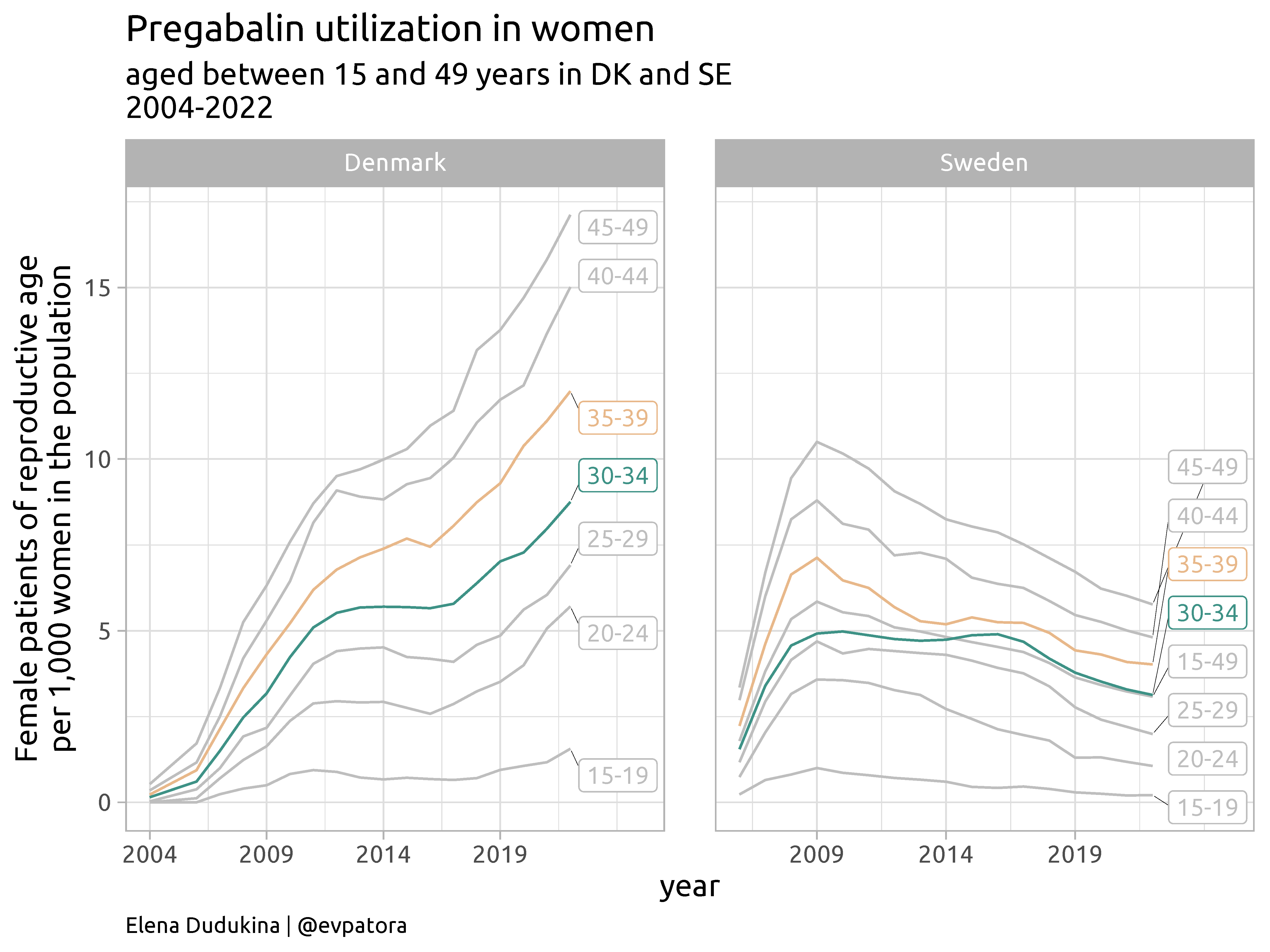
Country-level data on pregabalin use in women
Pregabalin is an antiepileptic drug (AED), prescribed to approximately 0.5 per thousand pregnant women in Europe, with increasing use after 2010.
Pregabalin and neurodevelopment study in the Nordics
Setting
- Non-interventional study was a post-authorisation safety (PAS) study conducted as a commitment to the European Medicines Agency (EUPAS27339)
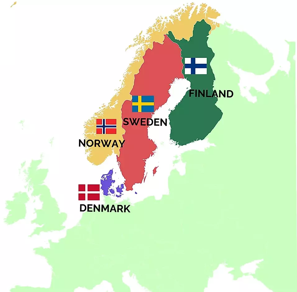
- Participants:
- Denmark
- Finland
- Sweden
- Norway
- Time period: 2005-2016
- Population-based
- All births identified in the respective medical birth registers from 01 January 2005 through 31 December 2015


Pregabalin and neurodevelopment study in the Nordics
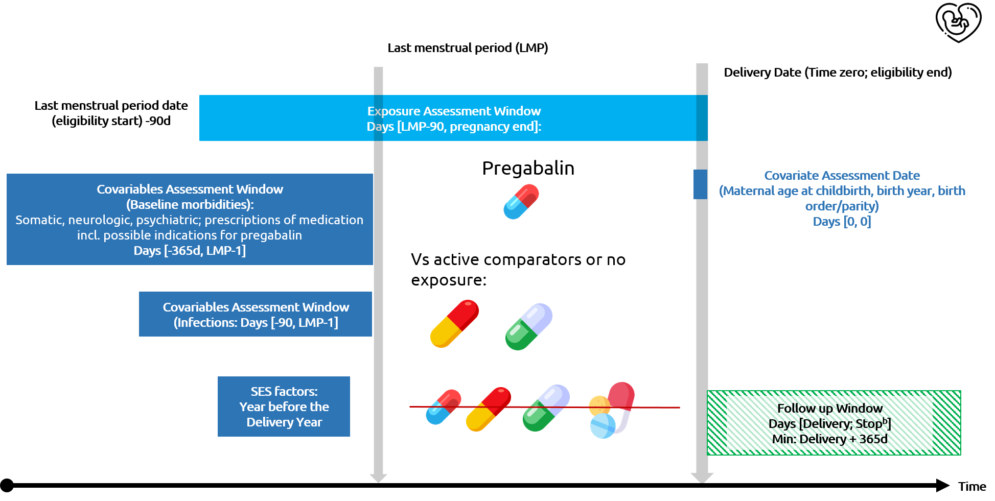
Exposure
- Any-trimester pregabalin exposure as at least one dispensing of pregabalin from LMP-90 days to the day before date of birth
- Pregabalin monotherapy in sensitivity analysis

Comparators
- No exposure to pregagbalin or other antiepileptics or active comparators
- Active comparators
- Lamotrigine
![]()
- Duloxetine
![]()
- Lamotrigine and/or duloxetine
![]() and/or
and/or ![]()
- Lamotrigine


Pregabalin and neurodevelopment study in the Nordics
Design
Pregabalin and neurodevelopment study in the Nordics
Covariables and confounding control


Pregabalin and neurodevelopment study in the Nordics
Covariables
- All covariables were available for at least 12 months before the end of the earliest identified pregnancy
- Maternal pre-pregnancy comorbidities using diagnostic codes from the national patient registries
- Maternal pre-pregnancy medication use from the national prescription registers
Pregabalin and neurodevelopment study in the Nordics
Descriptive variables:
- Caesarean delivery
![]()
- Children’s sex distributions
![]()
- Distributions of potential indications for pregabalin use inferred by recorded diagnoses before pregnancy (epilepsy, pain, GAD)


Pregabalin and neurodevelopment study in the Nordics
Postnatal outcomes
- Attention deficit/hyperactivity disorder (ADHD)
- Autism spectrum disorder (ASD)
- Intellectual disability


Pregabalin and neurodevelopment study in the Nordics
Main results
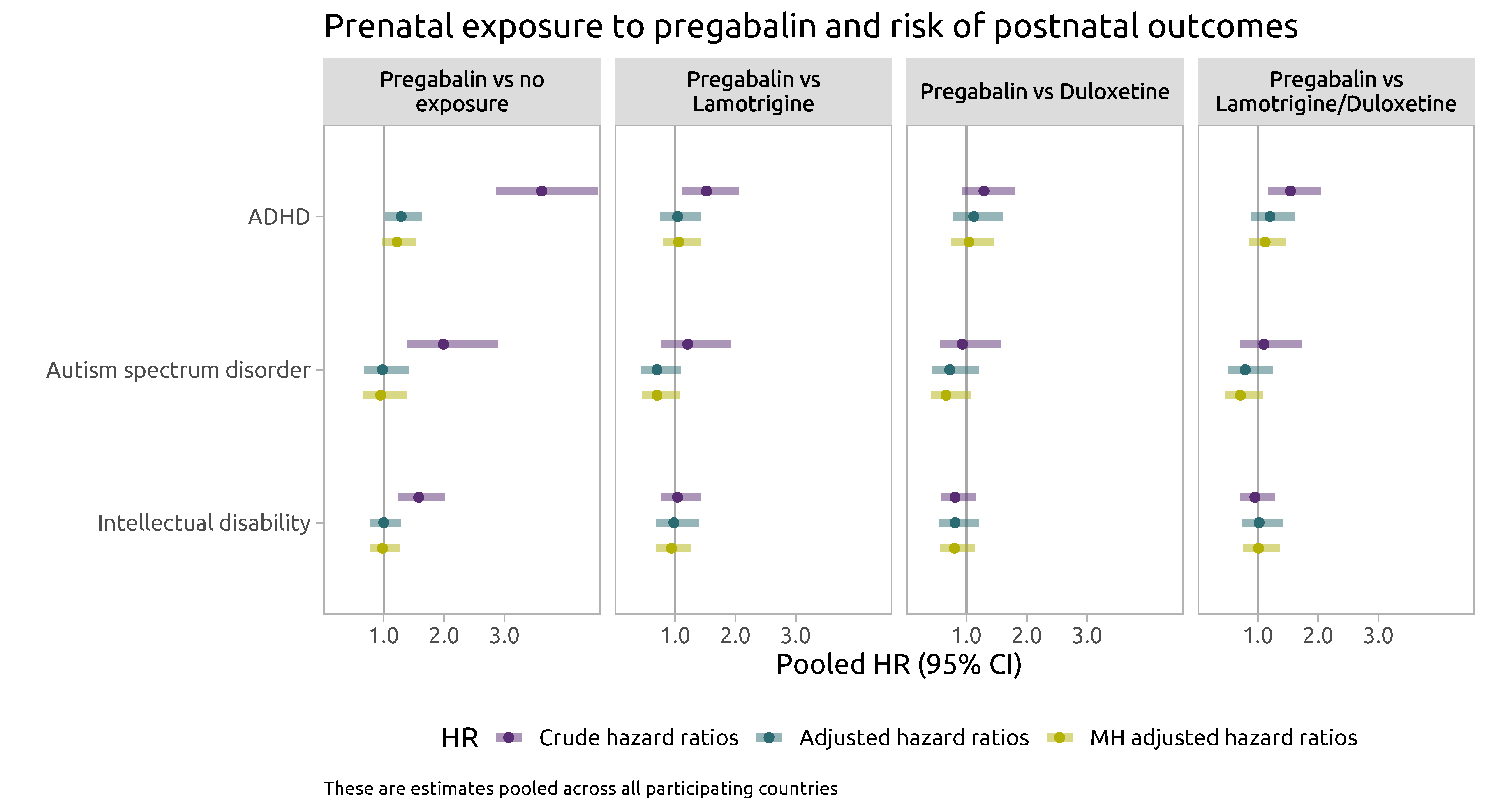
Pregabalin and neurodevelopment study in the Nordics
Additional results
Pregabalin and neurodevelopment study in the Nordics
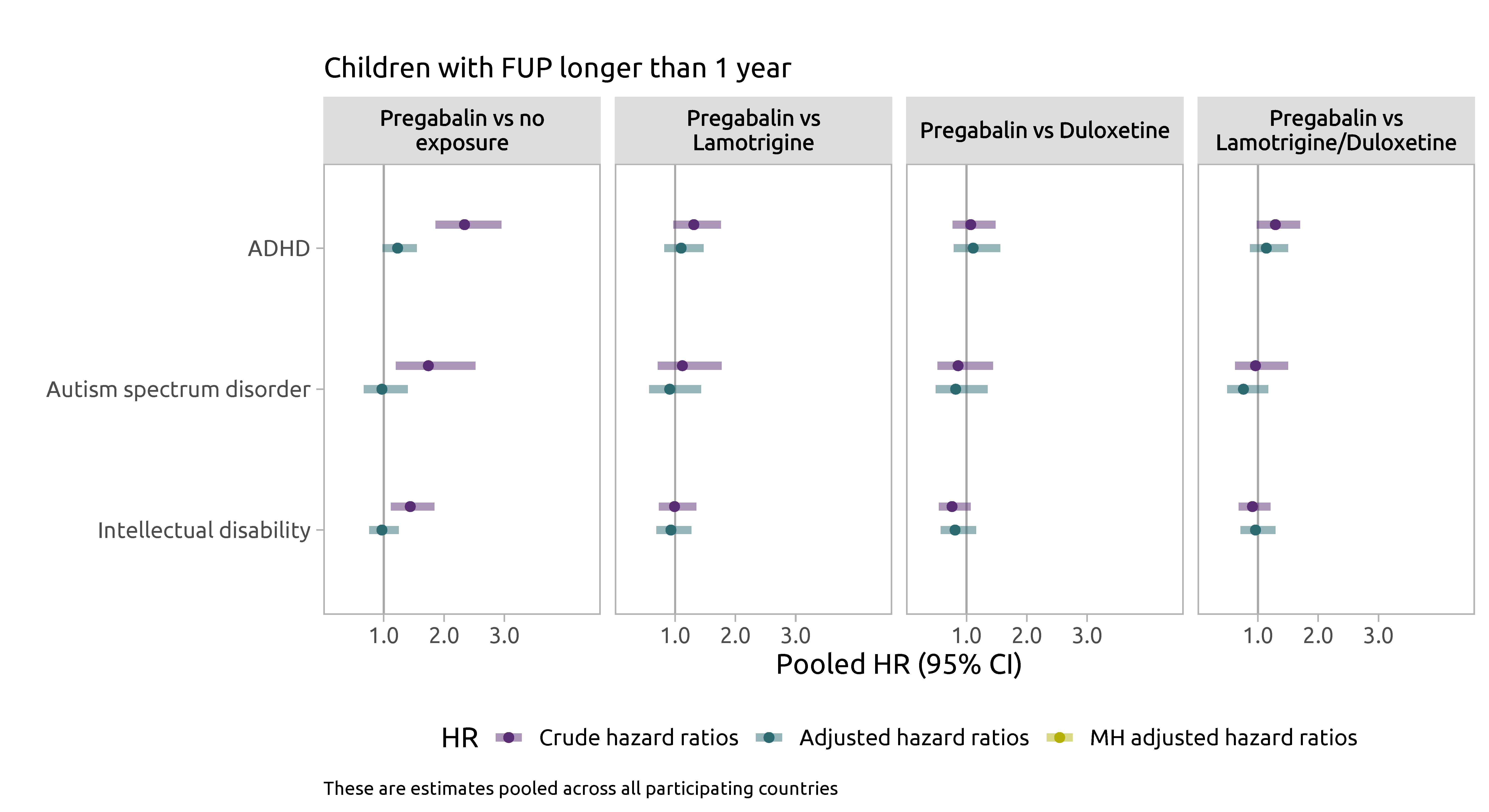
Monotherapy analyses
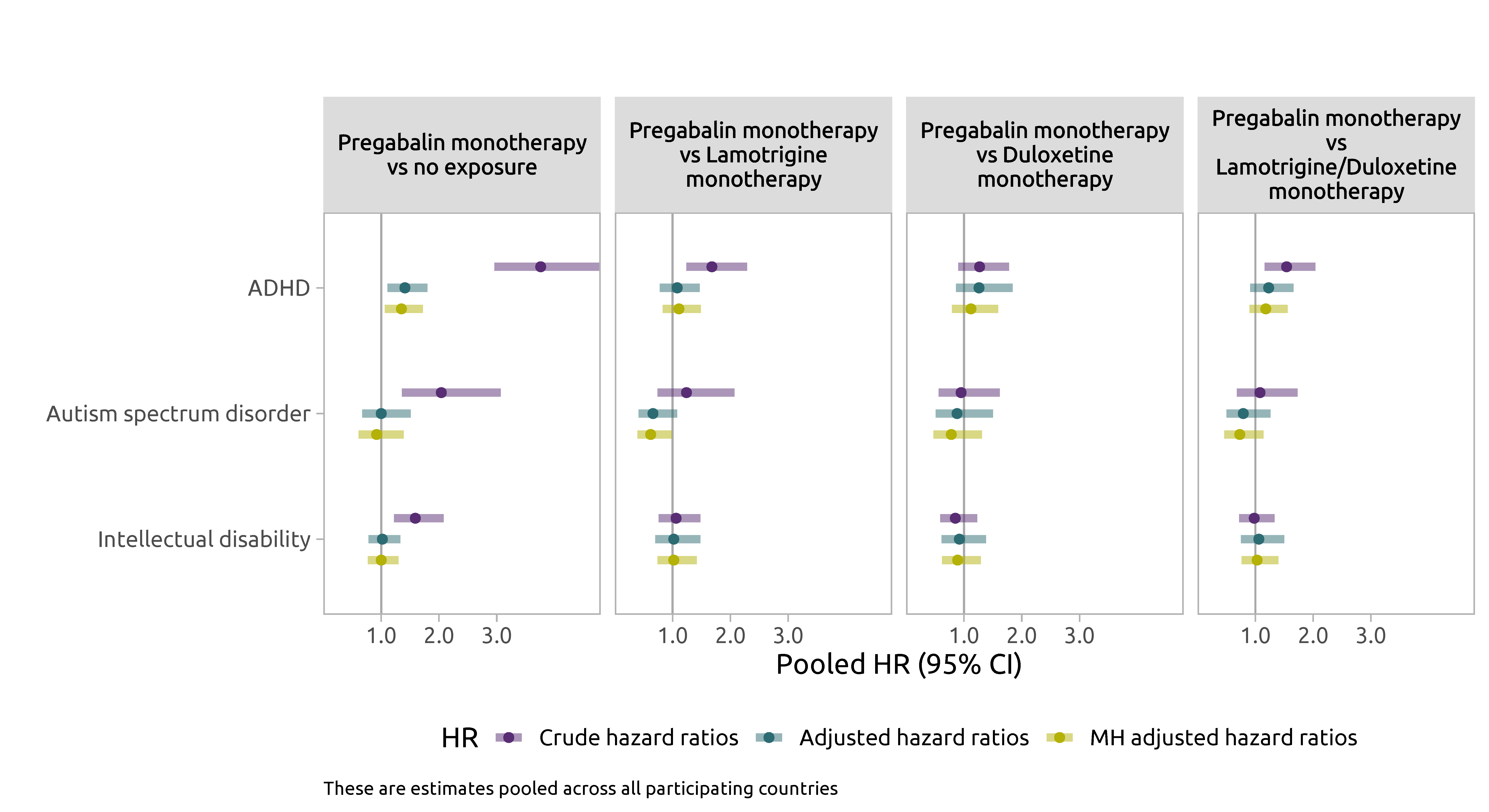
Pregabalin and neurodevelopment study in the Nordics
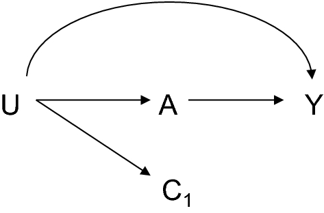
Residual confounding
- Unbalance for the contrast of offspring with exposure to pregabalin vs no exposure
![]()
- analgesics
- antipsychotics
- antidepressants
- history of depression and other neurological disorders
- Residual confounding by indication cannot be ruled out

Pregabalin and neurodevelopment study in the Nordics
Comparisons with previous studies
- Valproate is associated with 1.5-fold increased risk of ADHD and 2.4-fold increased risk of any postnatal neurodevelopmental disorder1
Pregabalin and neurodevelopment study in the Nordics
Outcome misclassification
- Few false-positives are expected
- Positive predictive values for ADHD coding 87% (DK)
- Positive predictive values for autism coding 94% (DK)
- Age at ADHD onset:
- 8 years in Denmark
- 7.5 years in Finland
- 10.5 years in Norway
- 12 years in Sweden
- Children with subdiagnostic symptoms

Pregabalin and neurodevelopment study in the Nordics
Exposure misclassification
- Possible: true intake of pregabalin and comparators is unknown
- Redeemed prescriptions > issued prescriptions

Conclusion
- Increased risks in excess of 1.8 were unlikely for ADHD
- There was no evidence of an association with other examined neurodevelopmental postnatal outcomes
- Overall more reassuring finding than not

![]()